How to Draw Plot R of Data Uploaded

When it comes to interpreting the globe and the enormous amount of data it is producing on a daily basis, Information Visualization becomes the most desirable way. Rather than screening huge Excel sheets, information technology is e'er better to visualize that data through charts and graphs, to gain meaningful insights.

R – Graph Plotting

The R Programming Language provides some easy and quick tools that let us convert our data into visually insightful elements like graphs.

Graph plotting in R is of ii types:

• One-dimensional Plotting: In 1-dimensional plotting, we plot 1 variable at a time. For example, we may plot a variable with the number of times each of its values occurred in the entire dataset (frequency). Then, it is not compared to any other variable of the dataset. These are the 4 major types of graphs that are used for Ane-dimensional assay –
  • Five Point Summary
  • Box Plotting
  • Histograms
  • Bar Plotting
• Two-dimensional Plotting: In two-dimensional plotting, we visualize and compare ane variable with respect to the other. For example, in a dataset of Air Quality measures, nosotros would similar to compare how the AQI varies with the temperature at a detail place. So, temperature and AQI are 2 different variables and nosotros wish to see how i changes with respect to the other. These are the iii major kinds of graphs used for such kinds of analysis –
  • Box Plotting
  • Histograms
  • Scatter plots

For the purpose of this article, we volition apply the default dataset (mtcars) that is provided past RStudio.

Loading the Data

Open RStudio (or R Terminal) and start by loading the dataset. Type these commands in the panel. This is a way to load the default datasets provided past R. (Any other dataset may also be downloaded and used)

R

library (datasets)

data (mtcars)

To check if the data is correctly loaded, nosotros run the following command on console:

R

Output:

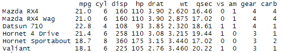
By running this command, we likewise get to know what columns does our dataset contains. In this case, the dataset mtcars contains eleven columns namely – mpg, cyl, disp, hp, drat, wt, qsec, vs, am, gear, and carb. Note that the number of rows is larger than displayed here. head() function displays only the top half-dozen rows of the dataset.

One-Dimensional Plotting

In i-dimensional plotting, nosotros essentially plot one variable at a time. So, it is non compared to whatever other variable of the dataset. Rather, only its features of statistical inference are taken care of.

V Signal Summary

To reference a particular column proper name in R, nosotros use the '$' sign. For example, if we want to refer to the 'gear' column in the mtcars dataset, we refer to it as – mtcars$gear. So, for whatsoever particular column of the dataset, we tin generate a Five-Point summary using the summary() office. We simply pass the cavalcade name (referred using $ sign) equally an argument to this part, as follows:

R

Output:

This summary lists down features similar Mean, Median, Minimum Value, Maximum Value, and Quadrant values of the particular cavalcade.

Box Plotting

A box plot generates a rectangle that covers the area spanned past the column of the dataset. Information technology can be produced every bit follows:

R

boxplot (mtcars$mpg, col= "light-green" )

Output:

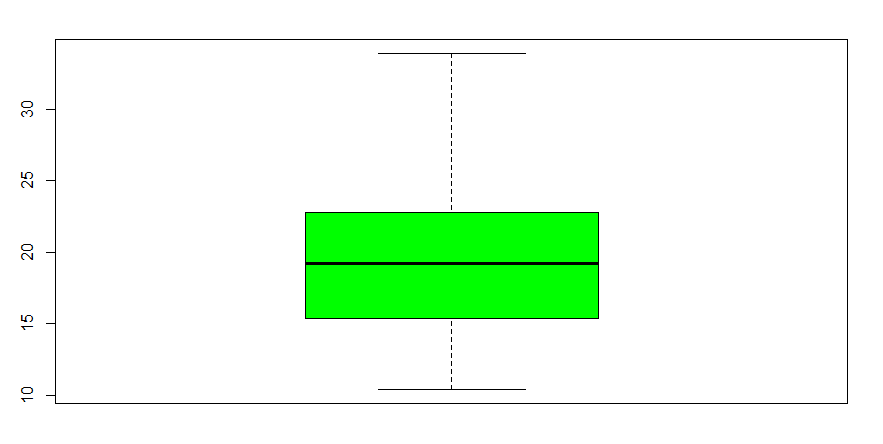
Note that the thick line in the rectangle depicts the median of the mpg column, i.e. 19.20 as seen in the 5 Point Summary. The col="green" simply colors the plot dark-green.

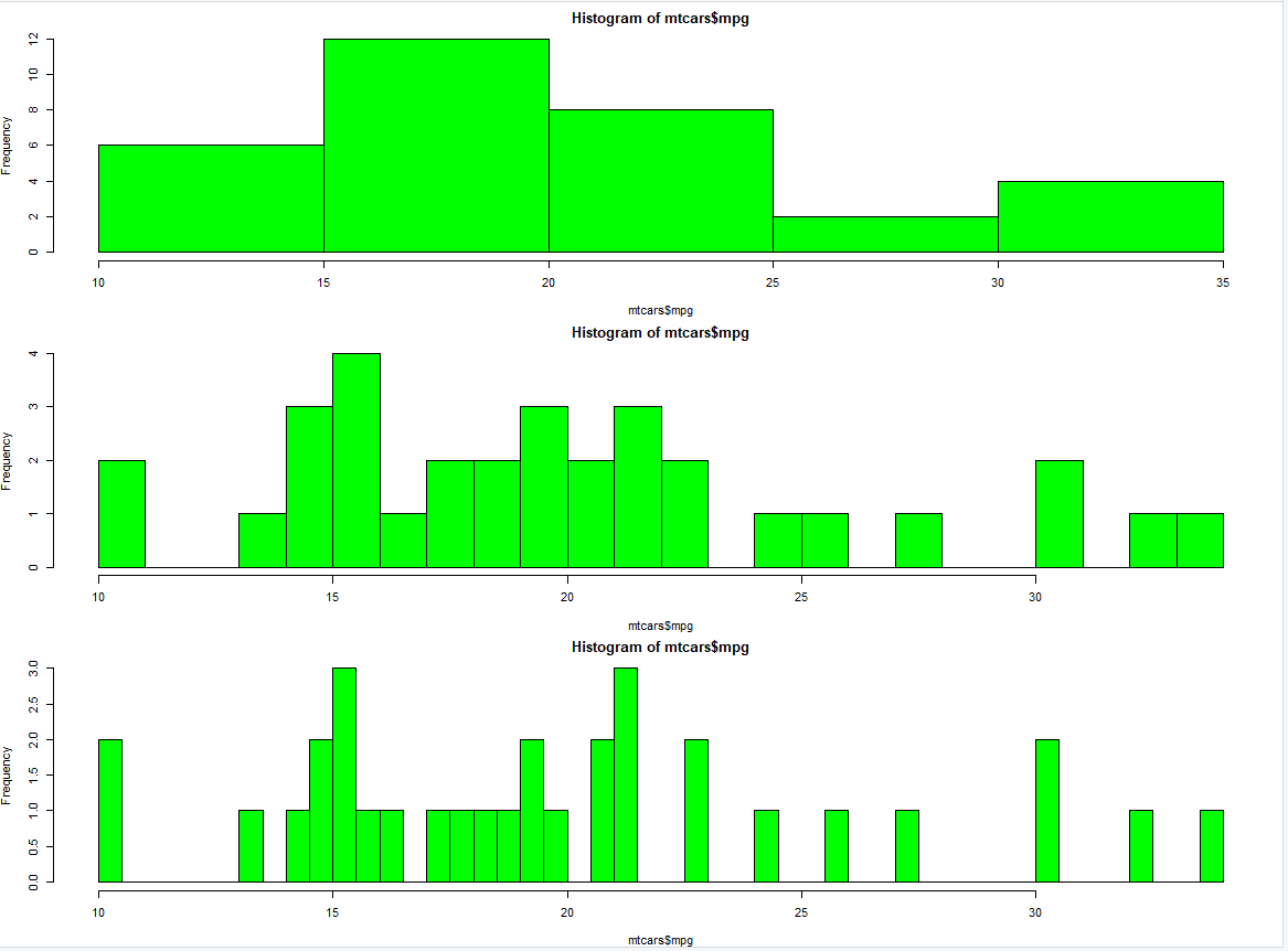
Histograms

Histograms are the nearly widely used plots for analyzing datasets. Here is how we tin plot a histogram that maps a variable (column proper name) to its frequency:

R

hist (mtcars$mpg, col = "dark-green" )

hist (mtcars$mpg, col = "greenish" , breaks = 25)

hist (mtcars$mpg, col = "dark-green" , breaks = l)

The 'breaks' argument essentially alters the width of the histogram bars. Information technology is seen that as nosotros increase the value of the break, the bars abound thinner.

Outputs:

Bar Plotting

In bar graphs, we get a discrete value-frequency mapping for each value present in the variable (column). For example:

R

barplot ( table (mtcars$carb), col= "green" )

Output:

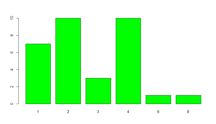
We run across that the column 'carb' contains half dozen discrete values (in all its rows). The above bar graph maps these six values to their frequency (the number of times they occur).

2-Dimensional Plotting

In two-dimensional plotting, nosotros visualize and compare one variable with respect to the other.

Box Plotting

Suppose nosotros wish to generate multiple boxplots, on the basis of the number of gears that each car has. So, the number of boxplots nosotros wish to have is equal to the number of discrete values in the column 'gear', i.e. one plot for each value of the gear. This tin can exist achieved in the post-obit way –

R

boxplot (mpg~gear, information=mtcars, col = "greenish" )

Output:

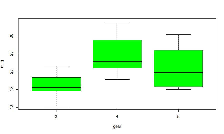
We run into that there are 3 values of gears in the 'gear' cavalcade. And then, 3 different box-plots, i for each gear have been plotted.

Histograms

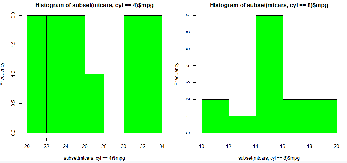
Now suppose, we wish to create carve up histograms for cars that have four cylinders and cars that have eight cylinders. To exercise this, nosotros subset our dataset such that the subset information contains information merely for those cars which have 4 (or 8) cylinders. Then, we tin can easily plot our subset data using hist() part as earlier. This is how we can achieve this:

R

hist ( subset (mtcars, cyl == 4)$mpg, col = "green" )

hist ( subset (mtcars, cyl == viii)$mpg, col = "green" )

Besprinkle Plot

Besprinkle plots are used to plot data points for two variables on the x and y-axis. They tell us patterns among data and are widely used for modeling ML algorithms. Hither, nosotros scatter plot the column qsec with respect to the column mpg.

R

with (mtcars, plot (mpg, qsec))

Output:

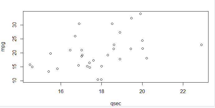
However, the above plot does not really bear witness u.s. any patterns in information. This is because of the limited number of rows (samples) we had in our dataset. When nosotros obtain data from external resources, it normally has a minimum of chiliad+ rows. On plotting such an extensive dataset on a scatter plot, we pave way for really interesting observations and insights.

carrollgrevinat.blogspot.com

Source: https://www.geeksforgeeks.org/graph-plotting-in-r-programming/